What is Random?

As previously discussed, there's no universal measure of randomness. Randomness implies the lack of pattern and the inability to predict future outcomes. However, The lack of an obvious model doesn't imply randomness anymore than a curve fit one implies order. So what actually constitutes randomness, how can we quantify it, and why do we care?

Randomness $\neq$ Volatility, and Predictability $\neq$ Profit

First off, it's important to note that predictability doesn't guarantee profit. On short timescales structure appears, and it's relatively easy to make short term predictions on the limit order book. However, these inefficiencies are often too small to capitalize on after taking into account commissions. Apparent arbitrage opportunities may persist for some time as the cost of removing the arb is larger than the payout.

Second, randomness and volatility are oft-used interchangeably in the same way that precision and accuracy receive the same colloquial treatment. Each means something on its own, and merits consideration as such. In the example above, predictability does not imply profitability anymore than that randomness precludes it. Take subprime for example – the fundamental breakdown in pricing and risk control resulted from correlation and structure, not the lack thereof.

Quantifying Randomness

Information theory addresses the big questions of what is information, and what are the fundamental limits on it. Within that scope, randomness plays an integral role in answering questions such as "how much information is contained in a system of two correlated, random variables?" A key concept within information theory is Shannon Entropy – a measure of how much uncertainty there is in the outcome of a random variable. As a simple example, when flipping a weighted coin, entropy is maximized when the probability of heads or tails is equal. If the probability of heads or tails is .9 and .1 respectively, the variable is still random, but guessing heads is a much better bet. Consequently, there's less entropy in the distribution of binary outcomes for a weighted coin flip than there is for a fair one. The uniform distribution is a so called maximum entropy probability distribution as there's no other continuous distribution with the same domain and more uncertainty. With the normal distribution you're reasonably sure that the next value won't be far away from the mean on one of the tails, but the uniform distribution contains no such information.

There's a deep connection between entropy and compressibility. Algorithms such as DEFLATE exploit patterns in data to compress the original file to a smaller size. Perfectly random strings aren't compressible, so is compressibility a measure of randomness? Kolmogorov complexity measures, informally speaking, the shortest algorithm necessary to describe a string. For a perfectly random source, compression will actually increase the length of the string as we'll end up with the original string (the source in this case is its own shortest description) along with the overhead of the compression algorithm. Sounds good, but there's one slight problem – Kolmogorov complexity is an uncomputable function. In the general case, the search space for an ideal compressor is infinite, so while measuring randomness via compressibility kind of works, it's always possible that a compression algorithm exists for which our source is highly compressible, implying that the input isn't so random after all.

What about testing for randomness using the same tools used to assess the quality of a random number generator? NIST offers a test suite for doing so. However, there are several problems with this approach. For starters, these tests need lots of input – 100,000+ data points. Even for high frequency data that makes for a very backward looking measure. Furthermore, the tests are designed for uniformly distributed sample data. We could use the probability integral transform to map our sample from some (potentially empirical) source distribution to the uniform distribution, but now we're stacking assumptions on top of heuristics.

Visualizing Volatility and Entropy

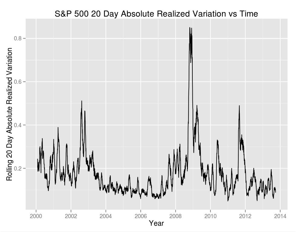
Of the above it sounds like entropy gets us the closest to what we want, so let's see what it looks like compared to volatility. We'll start by plotting the 20 day trailing absolute realized variation of the S&P 500 cash index as a measure of volatility:

1
2
3
4
5
6
7
8
9
10
11
12
13
14
15
16
17
18
19
20
21
22
23
require(quantmod)
require(ggplot2)
require(TTR)

# Calculate open to close log returns on the S&P 500 cash index
sp.data <- dailyReturn(getSymbols("^GSPC", env = .GlobalEnv, 
	from = "2000-01-01", to = "2013-09-27", src = "yahoo", 
	auto.assign = FALSE), type = "log")

# Calculate a rolling 20 day absolute realized variation over the returns
sp.arv20 <- tail(runSum(abs(sp.data), n = 20), -19)
sp.arv20.df <- data.frame(
	Date = as.Date(index(sp.arv20)),
	ARV = as.vector(sp.arv20))

# Plot our results
ggplot(sp.arv20.df, aes(x = Date, y = ARV)) +
	geom_line() +
	theme(plot.background = element_rect(fill = '#F1F1F1'),
		legend.background = element_rect(fill = '#F1F1F1')) +
	xlab("Year") +
	ylab("Rolling 20 Day Absolute Realized Variation") +
	ggtitle("S&P 500 20 Day Absolute Realized Variation vs Time")

Now let's look at entropy. Entropy is a property of a random variable, and as such there's no way to measure the entropy of data directly. However, if we concern ourselves only with the randomness of up/down moves there's an easy solution. We treat daily returns as Bernoulli trials in which a positive or a zero return is a one and a negative return is a 0. We could use a ternary alphabet in which up, down, and flat are treated separately, but seeing as there were only two flat days in this series doing so only obfuscates the bigger picture.

1
2
3
4
5
6
7
8
9
10
11
12
13
14
15
16
17
18
19
20
21
22
23
24
25
26
27
28
# Shannon entropy of the Bernoulli distribution
shannon.entropy <- function(x) {
	len <- length(x)
	p.up <- sum(x >= 0) / len
	p.down <- sum(x < 0) / len
	total <- 0
	if(p.up > 0)
	{
		total <- total + p.up * log(p.up, 2)
	}
	if(p.down > 0)
	{
		total <- total + p.down * log(p.down, 2)
	}
	return(-total)
}

sp.entropy20 <- tail(rollapply(sp.data, 20, shannon.entropy), -19)
sp.entropy20.df <- data.frame(
	Date = as.Date(index(sp.entropy20)),
	Entropy = as.vector(sp.entropy20))
ggplot(sp.entropy20.df, aes(x = Date, y = Entropy)) +
	geom_line() +
	theme(plot.background = element_rect(fill = '#F1F1F1'),
		legend.background = element_rect(fill = '#F1F1F1')) +
	xlab("Year") +
	ylab("Rolling 20 Day Shannon Entropy") +
	ggtitle("S&P 500 Rolling 20 Day Shannon Entropy vs Time")

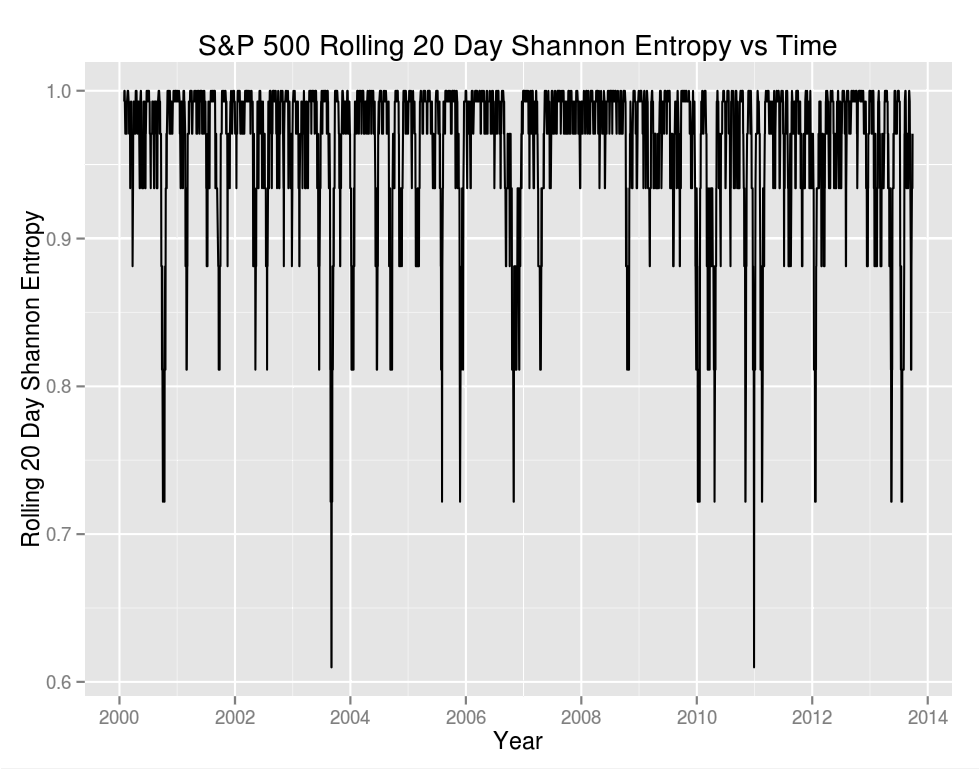
Visually the two plots look very different. We see that most of the time $H(X)$ is close to one (the mean is .96), indicating that our "coin" is fair and that the probability of a day being positive or negative over a trailing 20 day period is close to .5.

How correlated are the results? If we consider the series directly we find that $Cor(H(X),\ \sigma) = .095$. It might be more interesting to consider the frequency in which an increase in volatility is accompanied by an increase in entropy: .500 – spot on random. Entropy and volatility are distinct concepts.

In Closing…

The reoccurring theme of "what are we actually trying to measure," in this case randomness, isn't trivial. Any metric, indicator, or computed value is only as good as the assumptions that went into it. For example, in the frequentist view of probability, a forecaster $F(X|x_{t-1}, \ldots, x_0)$ is "well calibrated" if the true proportion of outcomes $X = x$ is close to the forecasted proportion of outcomes (there's a Bayesian interpretation as well but the frequentist one is more obvious). It's possible to cook up a forecaster that's wrong 100% of the time, but spot on with the overall proportion. That's horrible when you're trying to predict if tomorrow's trading session will be up or down, but terrific if you're only interested in the long term proportion of up and down days. As such, discussing randomness, volatility, entropy, or whatever else may be interesting from an academic standpoint, but profitability is a whole other beast, and measuring something in distribution is inherently backward looking.

Waiting Sucks.

Queuing effects arise daily. From optimizing traffic flow in Los Angeles to multitasking on your iPhone, queues and the techniques used to model them make the world a better place. Whenever there's contention for a finite pool of resources, you have a queue. Queues come in many flavors and disciplines for how tasks are added and serviced, but at the end of the day the question is the same: how do you efficiently allocate resources to consumers, under some set of constraints?

In high frequency trading, variability in response time is at least as important as mean response time. If you have a known and stable mean response time you're better able to model which trades are actually feasible. Depending on the trade, you might require that your system provide real-time responses, either hard of soft. At that level, variance in everything from the system clock to the ring buffer that the network card uses to handle incoming packets matters. It's important to profile these components individually and as a whole to understand how the system will respond to a given load.

Task Schedulers to the Rescue…?

In a CPU, you'll likely have more threads and processes (consumers) than you have CPU cores (resources). Even if your CPU utilization is light, lots of little background tasks need to run periodically, and programs rely on threads to respond to user input immediately even when they're doing some work in the background. Threads are abstractions but CPU cores are bare metal. In practice, modern CPU cores have some level of parallelism in the form of speculative execution and instruction reordering, but the general contract holds that within a single thread, these effects cannot be visible.

To keep things civil when there are more threads than cores, modern OS kernels use preemptive multitasking. As opposed to forcing programs to explicitly cooperate and yield resources when they don't need them, the OS is free to halt the execution of a program, save its state, let something else run, and restart the paused program after restoring its previous state. All of this is transparent to the program – the contract that a single thread must see its own memory effects in order remains intact.

All of that sounds great, but OS task scheduling, along with locking in multi threaded programs, are two of the biggest enemies of real-time computing. Both have queuing effects, either explicit or implicit. Let's consider the Linux scheduler. In Linux, threads and processes receive the same treatment when it comes to scheduling: a process is viewed as a single thread which can in turn own multiple threads. For simplicity we'll refer to work being scheduled as a task, and the time that it's allotted as a time slice. The default scheduler since 2.6.23 is the completely fair scheduler (CFS). There are a multitude of ways to implement a scheduler but as the name alludes to, the CFS attempts to schedule processor time "fairly." Tasks that don't frequently utilize the CPU receive the highest priority when they request CPU time, preempting processor hogs. This fairly amortizes delay across tasks as long running/heavy utilization tasks have a small delay relative to their total utilization, and short lived tasks are delayed as little as possible when they do need CPU cycles.

Other types of schedulers use run queues (either per CPU core or across all cores), and both approaches have merits. The CFS does a better job of ensuring efficient utilization and preventing "worst case" behavior, at the cost of determinism. Unfortunately, your task may get preempted at a very inopportune time, like when you're trying to arb the second leg of a trade. The CFS delivers a good user experience for most workloads and prevents resource starvation issues – even at 100% CPU utilization the kernel can start a new process with minimal delay and reallocate resources. Real-time schedulers need a good deal of tuning from the system administrator, usually have a slightly worse mean response time, and only benefit specialized workloads. As such the CFS was chosen as a default.

Regardless of what scheduler you use, under constrained resources queuing effects will come into play, so let's dive into the math. In queuing theory systems are often denoted using Kendall's Notation and we'll do the same. As a first order approximation you could call the kernel scheduler an M/M/c queue, meaning that the arrival process is Poisson, service times are distributed exponentially, and c agents (cores) are available to process requests. When using locks the situation is a little different - a mutex is essentially an M/M/1 queue. Queuing theory has lots to offer and at some point I might write about its applications outside of scheduling, the limit order book being the obvious one. However, all we really need for now is a discussion of the arrival and wait time distributions.

Building a Stochastic Model

We need a few process models to describe the arrival of tasks to the scheduler, and how long it takes for a task to run. The Poisson process enjoys wide use as a model of physical processes with an "intensity," such as the arrival of customers to a store, or radioactive decay. It's Markovian, meaning that the current state of a system suffices to describe the system in entirety, and that the past doesn't effect future outcomes. For example, if fifty customers arrived at a store per hour (on average), we might model this as homogeneous Poisson. When calculating the probability that $k$ customers will arrive over some time window $[t_0,t_1]$ during the day we need only consider the average rate of arrival $\lambda = 50$ and the time window in question. We can even make $\lambda$ a function of time (it's reasonable that certain times of the day are busier than others).

There are three equivalent ways of defining a Poisson process, two of which are especially relevant to what we're discussing.

• A process in which the number of arrivals $N(t)$ over some finite period of time obeys a Poisson distribution $f(n; \lambda t)$
• A process in which the intervals of time between events are independent, and obey the exponential distribution

The equivalence of these statements makes for some slick applications of the Poisson process. For one, it implies that we can work directly with the exponential and Poisson distributions, both of which happen to have some especially nice properties. It's unrealistic to believe that arrival events are uncorrelated (network traffic and market data comes in bursts) or that run times are exponentially distributed, but as a first pass and without specific knowledge of the workload it's not a bad approximation.

Let's write a little code to see these stochastic effects in action:

1
2
3
4
5
6
7
8
9
10
11
12
13
14
15
16
17
18
19
20
21
22
23
24
25
26
27
28
29
30
31
32
33
34
35
36
37
38
39
40
41
42
43
44
45
46
47
48
49
50
51
52
53
54
55
56
57
58
59
60
61
#include <iostream>
#include <inttypes.h>
#include <cstdio>
#include <time.h>

using namespace std;

 __attribute__((always_inline))
timespec diff(timespec start, timespec end);

 __attribute__((always_inline))
int64_t hash(int64_t a);
 
int main()
{
	int runCount = 100000;
	timespec startTime, endTime, timeDelta;
	int64_t deltas[runCount];
	clock_gettime(CLOCK_PROCESS_CPUTIME_ID, &startTime);
	int64_t a = startTime.tv_nsec;	
	
	for (int i = 0; i < runCount; i++) {
		clock_gettime(CLOCK_PROCESS_CPUTIME_ID, &startTime);
		a = hash(a);
		clock_gettime(CLOCK_PROCESS_CPUTIME_ID, &endTime);
		timeDelta = diff(startTime, endTime);
		deltas[i] = 1000000000 * timeDelta.tv_sec + timeDelta.tv_nsec;
	}

	for (int i = 0; i < runCount; i++) {
		cout << deltas[i] << endl;
	}
	
	return 0;
}
 
timespec diff(timespec start, timespec end)
{
	timespec t;
	if ((end.tv_nsec - start.tv_nsec) < 0) {
		t.tv_sec = end.tv_sec - start.tv_sec - 1;
		t.tv_nsec = 1000000000 + end.tv_nsec - start.tv_nsec;
	} else {
		t.tv_sec = end.tv_sec - start.tv_sec;
		t.tv_nsec = end.tv_nsec - start.tv_nsec;
	}
	return t;
}

int64_t hash(int64_t a) {
    for(int i = 0; i < 64; ++i) {
        a -= (a << 6);
        a ^= (a >> 17);
        a -= (a << 9);
        a ^= (a << 4);
        a -= (a << 3);
        a ^= (a << 10);
        a ^= (a >> 15);
    }
    return a;
}

## Fat Tails

I ran the given code pegged to a single core on a box with 100% CPU utilization. Obviously there are lots of sources of randomness in play – the main goal was to demonstrate:

1. For a deterministic function, controlling for other sources of variability, evaluation times are approximately exponentially distributed.
2. The scheduler will periodically preempt execution execution of our thread, resulting in huge spikes in latency.

As for the results:

There are some minor peaks after the big one but the exponential drop off is pronounced. It's a little more clear from the empirical cumulative distribution function:

However, I neglected to mention that both of the images above are zoomed way, way in. The distribution, in entirety looks like:

Ouch. There's the scheduler jitter that we were discussing before. The tail on that graph is so far out that it's hardly worth showing. It's easier to consider a tabulated description. For 100,000 iterations:

• Mean: 2108.956ns
• Median: 2081ns
• SD: 1619.491ns
• Min: 979ns
• Max: 189,705ns
• Number of iterations > $\mu + 1\sigma$: 169
• Number of iterations > $\mu + 2\sigma$: 156
• Number of iterations > $\mu + 3\sigma$: 87
• Number of iterations > $\mu + 4\sigma$: 62
• Number of iterations > $\mu + 5\sigma$: 38
• Number of iterations > $\mu + 6\sigma$: 29
• Number of iterations > $\mu + 10\sigma$: 13
• Number of iterations > $\mu + 20\sigma$: 12
• Number of iterations > $\mu + 50\sigma$: 9
• Number of iterations > $\mu + 100\sigma$: 8

That's seriously bad news for a system with soft real-time requirements unless the requirement is a whopping $10\sigma$ from the mean. So what can be done? There are a few possibilities. For one, we can politely suggest to the scheduler that our thread is a very important one:

1
2
3
4
5
6
7
8
9
10
11
12
13
14
15
16
17
18
19
20
21
22
#include <pthread.h>
#include <sched.h>

bool set_realtime_priority() {
    int ret;
    pthread_t current_thread = pthread_self();
	struct sched_param params;
	params.sched_priority = sched_get_priority_max(SCHED_FIFO);
 
	ret = pthread_setschedparam(current_thread, SCHED_FIFO, &params);
	if (ret != 0) {
		return false;
	}

    int policy = 0;
    ret = pthread_getschedparam(current_thread, &policy, &params);
    if (ret != 0 || policy != SCHED_FIFO) {
        return false;
    }
 
    return true;
}

How well does it listen? Running the same test again including set_realtime_priority() gives:

• Mean: 2115.28
• Median: 2092.00
• SD: 1564.30
• Min: 2084.00
• Max: 188273.00
• Number of iterations > $\mu + 1\sigma$: 82
• Number of iterations > $\mu + 2\sigma$: 82
• Number of iterations > $\mu + 3\sigma$: 76
• Number of iterations > $\mu + 4\sigma$: 66
• Number of iterations > $\mu + 5\sigma$: 55
• Number of iterations > $\mu + 6\sigma$: 30
• Number of iterations > $\mu + 10\sigma$: 16
• Number of iterations > $\mu + 20\sigma$: 13
• Number of iterations > $\mu + 50\sigma$: 9
• Number of iterations > $\mu + 100\sigma$: 7

Interesting. Variance is reduced slightly and the distribution tightens up significantly in the one and two sigma range. However this does nothing for the tails. The fact remains that under full load something's gotta give, and the scheduler will happily ignore our suggestion. So what about the light load case?

Without using set_realtime_priority():

• Mean: 2121.37
• Median: 2092.00
• SD: 1663.52
• Min: 192.00
• Max: 185780.00
• Number of iterations > $\mu + 1\sigma$: 130
• Number of iterations > $\mu + 2\sigma$: 125
• Number of iterations > $\mu + 3\sigma$: 96
• Number of iterations > $\mu + 4\sigma$: 52
• Number of iterations > $\mu + 5\sigma$: 32
• Number of iterations > $\mu + 6\sigma$: 24
• Number of iterations > $\mu + 10\sigma$: 10
• Number of iterations > $\mu + 20\sigma$: 10
• Number of iterations > $\mu + 50\sigma$: 9
• Number of iterations > $\mu + 100\sigma$: 9

With set_realtime_priority():

• Mean: 2113.91
• Median: 2085.00
• SD: 1910.75
• Min: 2077.00
• Max: 176213.00
• Number of iterations > $\mu + 1\sigma$: 89
• Number of iterations > $\mu + 2\sigma$: 85
• Number of iterations > $\mu + 3\sigma$: 74
• Number of iterations > $\mu + 4\sigma$: 43
• Number of iterations > $\mu + 5\sigma$: 30
• Number of iterations > $\mu + 6\sigma$: 24
• Number of iterations > $\mu + 10\sigma$: 20
• Number of iterations > $\mu + 20\sigma$: 16
• Number of iterations > $\mu + 50\sigma$: 12
• Number of iterations > $\mu + 100\sigma$: 0

The Takeaway

It's clear that set_realtime_priority definitely helps to tighten the distribution around the mean, regardless of load. However, the fat tails persist as the scheduler is still free to preempt our task as required. There's lots of additional tuning that can be done to minimize these effects on commodity Linux, even without using a real-time kernel, but it's impossible to completely eliminate jitter in user space programs (or on commodity SMP hardware in general).

Real-time systems provide means of creating threads which cannot be preempted by the scheduler, and often have constructs for disabling hardware interrupts. When even those constructs don't cut it, ASICs and FPGAs offer true determinism as they operate on a fixed clock cycle. That's the nuclear option, and many companies such as Fixnetix have already gone down that rabbit hole.

Towards a Generic Factory

Architecting almost any large system requires loads of boilerplate code. Unfortunately, in the low latency space the adage that with powerful hardware a programmer's time outweights the program's efficiency doesn't hold.

Reflective capabilities and metaprogramming constructs are a godsend when it comes to programmer productivity. Rails and many other frameworks leverage them extensively to decouple implementation details from business logic and perform complex tasks such as persistence and transactions transparently. Though rife with potential for abusing anti patterns and creating maintenance nightmares, reflection proves extremely useful when used tastefully.

One such application is for a generic factory method returning instances of a given type – a trivial task repeated in codebases the world over. In java the pattern looks something like:

1
2
3
4
5
6
public interface Factory<T> {

    T create();


}

1
2
3
4
5
6
7
8
9
10
11
12
13
14
15
16
17
18
19
20
21
22
23
24
25
public class GenericFatory<T> implements Factory<T> {

    private final Constructor<T> ctor;

    public GenericFatory(Class<T> clazz) {
        try {
            ctor = clazz.getConstructor();
        } catch (Exception e) {
            throw new IllegalArgumentException("Unable to retrieve a zero " +
                    "argument constructor for the given type.", e);
        }
    }

    @Override
    public T create() {
        try {
            return ctor.newInstance();
        } catch (Exception e) {
            throw new IllegalStateException("Unable to reflectively " +
                    "instantiate a new instance.", e);
        }
    }


}

## The Problem

The above looks like a great solution to the boilerplate alternative of creating a factory for every type that you might need a factory for. For a messaging layer where instances of a message type are instantiated based on a type ID in the message's serialized form, littering your code base with factories that look like:

1
2
3
4
5
6
7
8
9
public class WidgetMessageFactory implements Factory<WidgetMessage> {

    @Override
    public WidgetMessage create() {
        return new WidgetMessage();
    }


}

for every message type isn't an appealing proposition from either a maintenance or a readability standpoint. However, that's exactly what you would do for latency critical applications, as reflection comes at a price. Reflection in modern java has little overhead once JIT kicks in; most of the articles floating around calling reflection "expensive" while discussing a 10x to 100x performance overhead pertain to the dark days before reflection underwent heavy optimization. That said, there's almost always some inefficiency in the form of indirection and extra instructions. When performance really matters, even a few percent worth of "convenience" overhead on a hot path isn't acceptable, so we're back to square one. Automated source code generation as part of the build process eases the pain of typing boilerplate for problems like this but fails to address code base clutter and maintainability concerns.

Run Time Code Generation

Can we have our metaprogramming cake and eat it too? In java (and most VM based languages) the answer is yes. As java loads classes dynamically at run time we can generate a class on the fly, instantiate an instance of our new type, and proceed with business as usual. There's no overhead assuming that the generated class contains bytecode similar to what javac would generate. Class loaders are agnostic to their source; at the end of the day, all classes are read as a stream of bytes. Generating a class on the fly and loading it isn't cheap, but for use cases where this happens once as part of an initialization procedure, code generation offers gains.

Short of dealing with the java class file format directly several fantastic libraries exist to do the heavy lifting. On the lowest level BECL and ASM allow for fine grained control over code generation while javassist and cglib work with heavy layers of abstraction. I chose javassist for this example as the task at hand doesn't require anything fancy and javassist's ability to process embedded snippets of java keeps things simple. That said, documentation on javassist is a little lean.

1
2
3
4
5
6
7
8
9
10
11
12
13
14
15
16
17
18
19
20
21
22
23
24
25
26
27
28
29
30
31
32
33
34
35
36
37
38
39
40
41
42
43
44
45
46
47
48
49
50
51
52
53
54
55
56
57
58
59
60
61
62
63
64
65
66
67
68
69
70
71
72
73
74
75
76
77
78
79
80
81
82
83
84
85
86
87
88
89
90
91
92
93
94
95
96
97
98
99
100
101
102
103
104
105
106
107
108
109
110
111
112
113
114
115
116
117
118
119
120
121
122
123
124
125
126
127
128
129
package codegen;

import javassist.ClassPool;
import javassist.CtClass;
import javassist.CtConstructor;
import javassist.CtMethod;

import java.util.concurrent.ConcurrentHashMap;
import java.util.concurrent.atomic.AtomicInteger;

/**
 * Creates an object factory for a given {@link Class} type using runtime code
 * generation. The factory object returned will invoke the given type's zero
 * argument constructor to return a new instance.
 *
 * @author Kelly Littlepage
 */
public class FactoryGenerator {

    /***
     * Used to guarantee the uniqueness of generated class names.
     */
    private static final AtomicInteger COUNTER = new AtomicInteger();

    /***
     * The class pool to use for all generated classes
     */
    private static final ClassPool CLASS_POOL = ClassPool.getDefault();

    private static final CtClass[] NO_ARGS = {};

    /***
     * Cache generated factories for future use.
     */
    private static final ConcurrentHashMap<Class<?>, Factory<?>>
            CLASS_FACTORY_MAP = new ConcurrentHashMap<>();

    /***
     * Gets or creates an instance of {@link Factory} for the given type.
     *
     *
     * @param clazz The {@link Class} of the object that the generated
     * {@link Factory} should return upon a call to {@link Factory#create()}.
     *
     * @return An instance of {@link Factory} for the given {@link Class}.
     */
    public static <T> Factory getFactory(Class<T> clazz) {
        Factory factory = CLASS_FACTORY_MAP.get(clazz);
        // We may end up recreating a factory if two threads call this method
        // at the same time. Doing so isn't an issue - we just end up
        // doing a little extra work for the corner case while providing lock
        // free reads under most circumstances.
        if(null == factory) {
            factory = createFactory(clazz);
            // Let the first write win
            final Factory previousFactory = CLASS_FACTORY_MAP.
                    putIfAbsent(clazz, factory);
            factory = null == previousFactory ? factory : previousFactory;
        }
        return factory;
    }

    @SuppressWarnings("unchecked")
    private static <T> Factory<T> createFactory(Class<T> clazz) {
        try {
            // Check that the class has a default zero argument constructor
            clazz.getConstructor();
        } catch (Exception e) {
            throw new IllegalArgumentException("No default constructor for " +
                    "the given class.");
        }
        try {
            final CtClass factoryClazz = CLASS_POOL.makeClass(
                    nameForType(clazz));

            factoryClazz.addInterface(
                    CLASS_POOL.get(Factory.class.getCanonicalName()));

            // Add a default, zero argument constructor to the generated class.
            final CtConstructor cons = new CtConstructor(NO_ARGS, factoryClazz);
            cons.setBody(";");
            factoryClazz.addConstructor(cons);

            // Implement the Factory#create() method. Note that the return type
            // is Object. Due to erasure the JVM doesn't take into account type
            // parameters at runtime, so the erasure signature of
            // Factory#create() returns Object.
            final CtMethod factoryMethod = CtMethod.make(
                    "public Object create() { return new " +
                            clazz.getCanonicalName() + "(); }", factoryClazz);
            factoryClazz.addMethod(factoryMethod);

            final Class<?> generated = factoryClazz.toClass();

            // Free the generated CtClass object from the pool. This will will
            // reduce our memory footprint as we won't be reusing the instance
            // in the future.
            factoryClazz.detach();
            return (Factory<T>) generated.newInstance();
        } catch (Exception e) {
            throw new RuntimeException(
                    "Unable to generate a proxy factory.", e);
        }
    }

    /***
     * Generate a unique name for the given class type.
     *
     * @param clazz The {@link Class} to generate a name for.
     *
     * @return A unique name for the given class type.
     */
    private static String nameForType(Class<?> clazz) {
        final StringBuilder sb = new StringBuilder(Factory.class.
                getCanonicalName());
        sb.append("$impl_");
        sb.append(clazz.getCanonicalName());
        sb.append("_");
        sb.append(COUNTER.getAndIncrement());
        return sb.toString();
    }

    private FactoryGenerator() {
        throw new IllegalAccessError("Uninstantiable class.");
    }


}

The magic happens in the #createFactory() - the rest is boilerplate to generate unique class names and cache factories for future use if another factory is requested for the same type.

The generated code (with a little help from javap) looks like:

1
2
3
4
5
6
7
8
9
10
11
12
13
14
public class codegen.Factory$impl_codegen.Main.TestClass_0 implements codegen.Factory {
  public codegen.Factory$impl_codegen.Main.TestClass_0();
    Code:
       0: aload_0       
       1: invokespecial #12                 // Method java/lang/Object."<init>":()V
       4: return        

  public java.lang.Object create();
    Code:
       0: new           #16                 // class codegen/Main$TestClass
       3: dup           
       4: invokespecial #17                 // Method codegen/Main$TestClass."<init>":()V
       7: areturn       
}

This is exactly what we would expect - four instructions in which an object is allocated, initialized, and returned. Let's look at what javac produces for a factory generated at compile time:

1
2
3
4
5
6
7
8
9
10
11
12
13
14
15
16
17
18
19
20
21
22
Compiled from "TestClassFactory.java"
public class codegen.TestClassFactory implements codegen.Factory<codegen.TestClass> {
  public codegen.TestClassFactory();
    Code:
       0: aload_0       
       1: invokespecial #1                  // Method java/lang/Object."<init>":()V
       4: return        

  public codegen.TestClass create();
    Code:
       0: new           #2                  // class codegen/TestClass
       3: dup           
       4: invokespecial #3                  // Method codegen/TestClass."<init>":()V
       7: areturn       

  public java.lang.Object create();
    Code:
       0: aload_0       
       1: invokevirtual #4                  // Method create:()Lcodegen/TestClass;
       4: areturn       
}

This code looks strange - two methods with the same signature and different return types, as writing a class with such method declarations is illegal under the Java 7 Language Specification (JLS). However, the Java 7 VM Spec (JVMS) contains no such restriction. Section 4.3.4 discusses signatures and the class file format for encoding information on generic and parameterized types. The JVM doesn't use this information, and as noted in the last paragraph:

Oracle's Java Virtual Machine implementation does not check the well-formedness of the signatures described in this subsection during loading or linking. Instead, these checks are deferred until the signatures are used by reflective methods, as specified in the API of Class and members of java.lang.reflect. Future versions of a Java Virtual Machine implementation may be required to perform some or all of these checks during loading or linking.

Given the above, javac is free to do as it pleases, provided that input complies with the JLS. Having two methods with the same return type doesn't hurt anything provided that the compiler is smart enough to figure out the appropriate call site bindings and that the reflective capabilities of the runtime can handle the identical signatures (which they do, by preferring the method with the stronger return type when methods are queried for by name).

There's some history here as generics were added with the goal of backward compatibility and as few changes to the runtime as possible. As such javac generates both methods and decides which method to call at compile time based upon available type information. It might be tempting to code generate the specific type but doing so will get you an AbstractMethodError at run time. The JVM doesn't know anything about our generic type so when referenced by interface it looks for a method on our generated class with the signature create()Ljava/lang/Object.

Results

How well are we rewarded for the extra effort? Running a benchmark timing 100,000,000 calls to Factory#create() yielded:

• Direct instantiation: Elapsed time: 10.50, ops/sec: 9,523,435.70
• Code Generation: Elapsed time: 10.44, ops/sec: 9,579,994.46
• Reflection: Elapsed time: 11.46, ops/sec: 8,726,687.95

Each benchmark was run in isolation on a warmed up JVM pinned to a single core on the Linux 3.10 kernel. Even with the aforementioned there's still enough randomness to a microbenchmark that code generation comes out on top of direct instantiation – in reality there's zero difference. However, code generation enjoys a stable 10% edge over reflection. The two takeaways are that: 1) reflection on modern java is pretty solid and 2) if you really care, code generation clears the pathway to clean architecture with zero performance compromises.