Queuing - Where Math Meets CS

Waiting Sucks.

Queuing effects arise daily. From optimizing traffic flow in Los Angeles to multitasking on your iPhone, queues and the techniques used to model them make the world a better place. Whenever there's contention for a finite pool of resources, you have a queue. Queues come in many flavors and disciplines for how tasks are added and serviced, but at the end of the day the question is the same: how do you efficiently allocate resources to consumers, under some set of constraints?

In high frequency trading, variability in response time is at least as important as mean response time. If you have a known and stable mean response time you're better able to model which trades are actually feasible. Depending on the trade, you might require that your system provide real-time responses, either hard of soft. At that level, variance in everything from the system clock to the ring buffer that the network card uses to handle incoming packets matters. It's important to profile these components individually and as a whole to understand how the system will respond to a given load.

Task Schedulers to the Rescue…?

In a CPU, you'll likely have more threads and processes (consumers) than you have CPU cores (resources). Even if your CPU utilization is light, lots of little background tasks need to run periodically, and programs rely on threads to respond to user input immediately even when they're doing some work in the background. Threads are abstractions but CPU cores are bare metal. In practice, modern CPU cores have some level of parallelism in the form of speculative execution and instruction reordering, but the general contract holds that within a single thread, these effects cannot be visible.

To keep things civil when there are more threads than cores, modern OS kernels use preemptive multitasking. As opposed to forcing programs to explicitly cooperate and yield resources when they don't need them, the OS is free to halt the execution of a program, save its state, let something else run, and restart the paused program after restoring its previous state. All of this is transparent to the program – the contract that a single thread must see its own memory effects in order remains intact.

All of that sounds great, but OS task scheduling, along with locking in multi threaded programs, are two of the biggest enemies of real-time computing. Both have queuing effects, either explicit or implicit. Let's consider the Linux scheduler. In Linux, threads and processes receive the same treatment when it comes to scheduling: a process is viewed as a single thread which can in turn own multiple threads. For simplicity we'll refer to work being scheduled as a task, and the time that it's allotted as a time slice. The default scheduler since 2.6.23 is the completely fair scheduler (CFS). There are a multitude of ways to implement a scheduler but as the name alludes to, the CFS attempts to schedule processor time "fairly." Tasks that don't frequently utilize the CPU receive the highest priority when they request CPU time, preempting processor hogs. This fairly amortizes delay across tasks as long running/heavy utilization tasks have a small delay relative to their total utilization, and short lived tasks are delayed as little as possible when they do need CPU cycles.

Other types of schedulers use run queues (either per CPU core or across all cores), and both approaches have merits. The CFS does a better job of ensuring efficient utilization and preventing "worst case" behavior, at the cost of determinism. Unfortunately, your task may get preempted at a very inopportune time, like when you're trying to arb the second leg of a trade. The CFS delivers a good user experience for most workloads and prevents resource starvation issues – even at 100% CPU utilization the kernel can start a new process with minimal delay and reallocate resources. Real-time schedulers need a good deal of tuning from the system administrator, usually have a slightly worse mean response time, and only benefit specialized workloads. As such the CFS was chosen as a default.

Regardless of what scheduler you use, under constrained resources queuing effects will come into play, so let's dive into the math. In queuing theory systems are often denoted using Kendall's Notation and we'll do the same. As a first order approximation you could call the kernel scheduler an M/M/c queue, meaning that the arrival process is Poisson, service times are distributed exponentially, and c agents (cores) are available to process requests. When using locks the situation is a little different - a mutex is essentially an M/M/1 queue. Queuing theory has lots to offer and at some point I might write about its applications outside of scheduling, the limit order book being the obvious one. However, all we really need for now is a discussion of the arrival and wait time distributions.

Building a Stochastic Model

We need a few process models to describe the arrival of tasks to the scheduler, and how long it takes for a task to run. The Poisson process enjoys wide use as a model of physical processes with an "intensity," such as the arrival of customers to a store, or radioactive decay. It's Markovian, meaning that the current state of a system suffices to describe the system in entirety, and that the past doesn't effect future outcomes. For example, if fifty customers arrived at a store per hour (on average), we might model this as homogeneous Poisson. When calculating the probability that $k$ customers will arrive over some time window $[t_0,t_1]$ during the day we need only consider the average rate of arrival $\lambda = 50$ and the time window in question. We can even make $\lambda$ a function of time (it's reasonable that certain times of the day are busier than others).

There are three equivalent ways of defining a Poisson process, two of which are especially relevant to what we're discussing.

A process in which the number of arrivals $N(t)$ over some finite period of time obeys a Poisson distribution $f(n; \lambda t)$
A process in which the intervals of time between events are independent, and obey the exponential distribution

The equivalence of these statements makes for some slick applications of the Poisson process. For one, it implies that we can work directly with the exponential and Poisson distributions, both of which happen to have some especially nice properties. It's unrealistic to believe that arrival events are uncorrelated (network traffic and market data comes in bursts) or that run times are exponentially distributed, but as a first pass and without specific knowledge of the workload it's not a bad approximation.

Let's write a little code to see these stochastic effects in action:

scheduler_test.cpp

1
2
3
4
5
6
7
8
9
10
11
12
13
14
15
16
17
18
19
20
21
22
23
24
25
26
27
28
29
30
31
32
33
34
35
36
37
38
39
40
41
42
43
44
45
46
47
48
49
50
51
52
53
54
55
56
57
58
59
60
61
#include <iostream>
#include <inttypes.h>
#include <cstdio>
#include <time.h>

using namespace std;

 __attribute__((always_inline))
timespec diff(timespec start, timespec end);

 __attribute__((always_inline))
int64_t hash(int64_t a);
 
int main()
{
	int runCount = 100000;
	timespec startTime, endTime, timeDelta;
	int64_t deltas[runCount];
	clock_gettime(CLOCK_PROCESS_CPUTIME_ID, &startTime);
	int64_t a = startTime.tv_nsec;	
	
	for (int i = 0; i < runCount; i++) {
		clock_gettime(CLOCK_PROCESS_CPUTIME_ID, &startTime);
		a = hash(a);
		clock_gettime(CLOCK_PROCESS_CPUTIME_ID, &endTime);
		timeDelta = diff(startTime, endTime);
		deltas[i] = 1000000000 * timeDelta.tv_sec + timeDelta.tv_nsec;
	}

	for (int i = 0; i < runCount; i++) {
		cout << deltas[i] << endl;
	}
	
	return 0;
}
 
timespec diff(timespec start, timespec end)
{
	timespec t;
	if ((end.tv_nsec - start.tv_nsec) < 0) {
		t.tv_sec = end.tv_sec - start.tv_sec - 1;
		t.tv_nsec = 1000000000 + end.tv_nsec - start.tv_nsec;
	} else {
		t.tv_sec = end.tv_sec - start.tv_sec;
		t.tv_nsec = end.tv_nsec - start.tv_nsec;
	}
	return t;
}

int64_t hash(int64_t a) {
    for(int i = 0; i < 64; ++i) {
        a -= (a << 6);
        a ^= (a >> 17);
        a -= (a << 9);
        a ^= (a << 4);
        a -= (a << 3);
        a ^= (a << 10);
        a ^= (a >> 15);
    }
    return a;
}

## Fat Tails

I ran the given code pegged to a single core on a box with 100% CPU utilization. Obviously there are lots of sources of randomness in play – the main goal was to demonstrate:

For a deterministic function, controlling for other sources of variability, evaluation times are approximately exponentially distributed.
The scheduler will periodically preempt execution execution of our thread, resulting in huge spikes in latency.

As for the results:

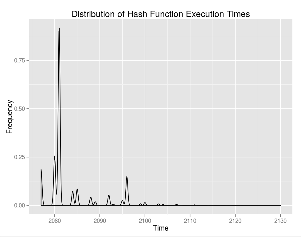
Hash function execution times zoomed

There are some minor peaks after the big one but the exponential drop off is pronounced. It's a little more clear from the empirical cumulative distribution function:

Hash function ecdf

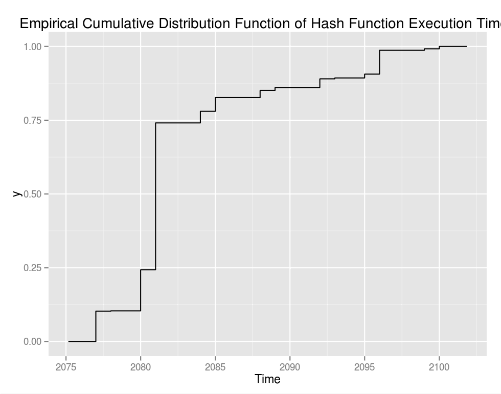
However, I neglected to mention that both of the images above are zoomed way, way in. The distribution, in entirety looks like:

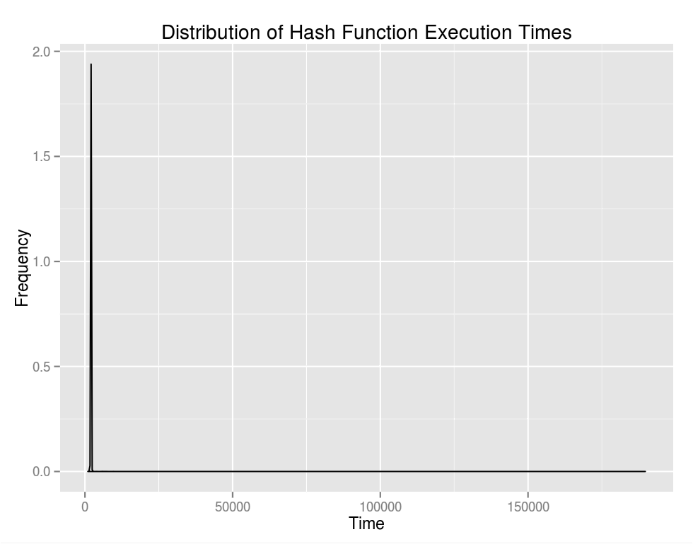
Hash function execution times full

Ouch. There's the scheduler jitter that we were discussing before. The tail on that graph is so far out that it's hardly worth showing. It's easier to consider a tabulated description. For 100,000 iterations:

Mean: 2108.956ns
Median: 2081ns
SD: 1619.491ns
Min: 979ns
Max: 189,705ns
Number of iterations > $\mu + 1\sigma$ : 169
Number of iterations > $\mu + 2\sigma$ : 156
Number of iterations > $\mu + 3\sigma$ : 87
Number of iterations > $\mu + 4\sigma$ : 62
Number of iterations > $\mu + 5\sigma$ : 38
Number of iterations > $\mu + 6\sigma$ : 29
Number of iterations > $\mu + 10\sigma$ : 13
Number of iterations > $\mu + 20\sigma$ : 12
Number of iterations > $\mu + 50\sigma$ : 9
Number of iterations > $\mu + 100\sigma$ : 8

That's seriously bad news for a system with soft real-time requirements unless the requirement is a whopping $10\sigma$ from the mean. So what can be done? There are a few possibilities. For one, we can politely suggest to the scheduler that our thread is a very important one:

1
2
3
4
5
6
7
8
9
10
11
12
13
14
15
16
17
18
19
20
21
22
#include <pthread.h>
#include <sched.h>

bool set_realtime_priority() {
    int ret;
    pthread_t current_thread = pthread_self();
	struct sched_param params;
	params.sched_priority = sched_get_priority_max(SCHED_FIFO);
 
	ret = pthread_setschedparam(current_thread, SCHED_FIFO, &params);
	if (ret != 0) {
		return false;
	}

    int policy = 0;
    ret = pthread_getschedparam(current_thread, &policy, &params);
    if (ret != 0 || policy != SCHED_FIFO) {
        return false;
    }
 
    return true;
}

How well does it listen? Running the same test again including set_realtime_priority() gives:

Mean: 2115.28
Median: 2092.00
SD: 1564.30
Min: 2084.00
Max: 188273.00
Number of iterations > $\mu + 1\sigma$ : 82
Number of iterations > $\mu + 2\sigma$ : 82
Number of iterations > $\mu + 3\sigma$ : 76
Number of iterations > $\mu + 4\sigma$ : 66
Number of iterations > $\mu + 5\sigma$ : 55
Number of iterations > $\mu + 6\sigma$ : 30
Number of iterations > $\mu + 10\sigma$ : 16
Number of iterations > $\mu + 20\sigma$ : 13
Number of iterations > $\mu + 50\sigma$ : 9
Number of iterations > $\mu + 100\sigma$ : 7

Interesting. Variance is reduced slightly and the distribution tightens up significantly in the one and two sigma range. However this does nothing for the tails. The fact remains that under full load something's gotta give, and the scheduler will happily ignore our suggestion. So what about the light load case?

Without using set_realtime_priority():

Mean: 2121.37
Median: 2092.00
SD: 1663.52
Min: 192.00
Max: 185780.00
Number of iterations > $\mu + 1\sigma$ : 130
Number of iterations > $\mu + 2\sigma$ : 125
Number of iterations > $\mu + 3\sigma$ : 96
Number of iterations > $\mu + 4\sigma$ : 52
Number of iterations > $\mu + 5\sigma$ : 32
Number of iterations > $\mu + 6\sigma$ : 24
Number of iterations > $\mu + 10\sigma$ : 10
Number of iterations > $\mu + 20\sigma$ : 10
Number of iterations > $\mu + 50\sigma$ : 9
Number of iterations > $\mu + 100\sigma$ : 9

With set_realtime_priority():

Mean: 2113.91
Median: 2085.00
SD: 1910.75
Min: 2077.00
Max: 176213.00
Number of iterations > $\mu + 1\sigma$ : 89
Number of iterations > $\mu + 2\sigma$ : 85
Number of iterations > $\mu + 3\sigma$ : 74
Number of iterations > $\mu + 4\sigma$ : 43
Number of iterations > $\mu + 5\sigma$ : 30
Number of iterations > $\mu + 6\sigma$ : 24
Number of iterations > $\mu + 10\sigma$ : 20
Number of iterations > $\mu + 20\sigma$ : 16
Number of iterations > $\mu + 50\sigma$ : 12
Number of iterations > $\mu + 100\sigma$ : 0

The Takeaway

It's clear that set_realtime_priority definitely helps to tighten the distribution around the mean, regardless of load. However, the fat tails persist as the scheduler is still free to preempt our task as required. There's lots of additional tuning that can be done to minimize these effects on commodity Linux, even without using a real-time kernel, but it's impossible to completely eliminate jitter in user space programs (or on commodity SMP hardware in general).

Real-time systems provide means of creating threads which cannot be preempted by the scheduler, and often have constructs for disabling hardware interrupts. When even those constructs don't cut it, ASICs and FPGAs offer true determinism as they operate on a fixed clock cycle. That's the nuclear option, and many companies such as Fixnetix have already gone down that rabbit hole.

Trading, Data Science, CS

Queuing - Where Math Meets CS

Waiting Sucks.

Task Schedulers to the Rescue…?

Building a Stochastic Model

The Takeaway

Comments